Offline tests
At the publication checkpoint, including the recorder recovery. Network access is denied during the Python test phase. The synthetic demo is explicitly invented data.
A better forecast is only the beginning of a trading strategy.
I built a research system for Texas electricity demand: correct the operator’s errors, model the range of possible peaks, then test whether an executable price can turn that information into value.
Forecast improvement measured.
Trading profitability unproven.
01 / THE FULL YEAR
Explore daily peak forecasts from the intraday experiment. Change the clock, model or month; the missing dates remain visible.
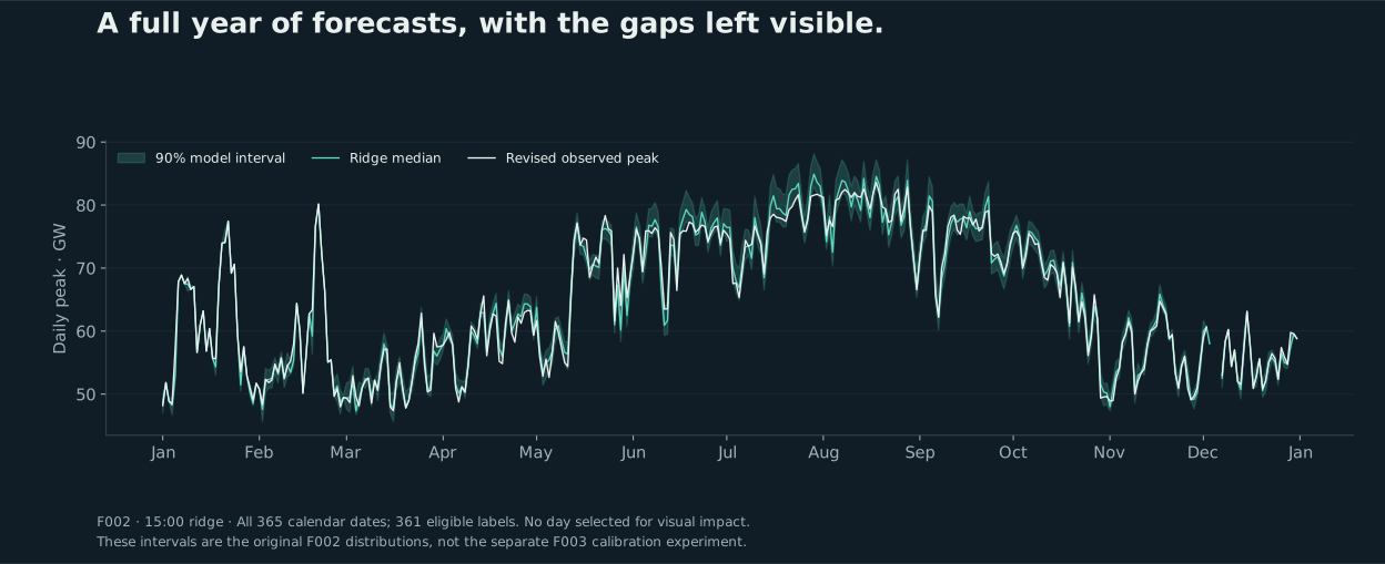
F002: 361 scored days out of 365 calendar dates.
| Date | Actual MW | Median MW | 90% range MW | Label |
|---|
F002 · These are forecasts of a revised EIA demand proxy, with assumed historical arrival clocks. They are not first-release ERCOT settlement forecasts or a price backtest. The displayed intervals are F002’s original distributions; the calibration experiment below uses separate, matched controls.
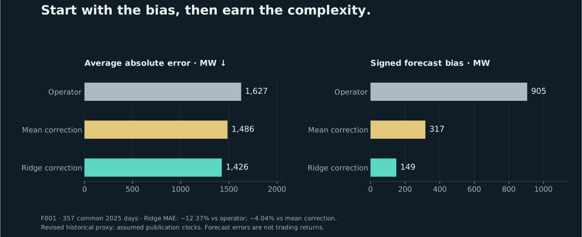
F001 ridge vs operator. 357 common days; 4.04% improvement over the stronger mean-correction baseline.
F002 ridge vs half update at 15:00. 361 days; descriptive comparison on an inspected development year.
F003 scaled ridge vs matched ridge at 14:00. A score that penalizes both wide ranges and missed outcomes.
Electricity demand has a useful starting point: the grid operator already publishes a forecast.
The first task was to estimate its remaining error. A model that learns persistent bias and incorporates the day’s observed trajectory can produce a distribution for the final daily peak.
The trading target is more specific: will the contract’s official hourly peak strictly exceed a threshold? The settlement source is ERCOT’s Actual System Load by Forecast Zone, NP6-346-CD. Revised EIA history is useful for model development, but it does not establish what that original release said.
This project grew out of WeatherPred, where better weather forecasts also failed to establish a trading edge. The energy work carries forward the timestamp, execution and validation lessons. Its implemented models are regression and residual scenarios; transformer and reinforcement-learning ideas are not energy results.
Archive inputs and actual receipt clocks.
Estimate the operator’s remaining error.
Keep whole hourly residual paths together.
Compare probabilities with executable asks.
Account for fills, fees, cash and settlement.
About 70% of the initial gain came from correcting average bias.
The raw operator peak had a +905 MW average bias in the common evaluation sample. Mean correction reduced that to +317 MW; ridge reduced it to +149 MW.
Ridge lowered mean absolute error from 1,627 to 1,426 MW. The relevant second comparison is 1,486 MW for mean correction. Complexity adds value here, but much less than the headline comparison alone suggests.
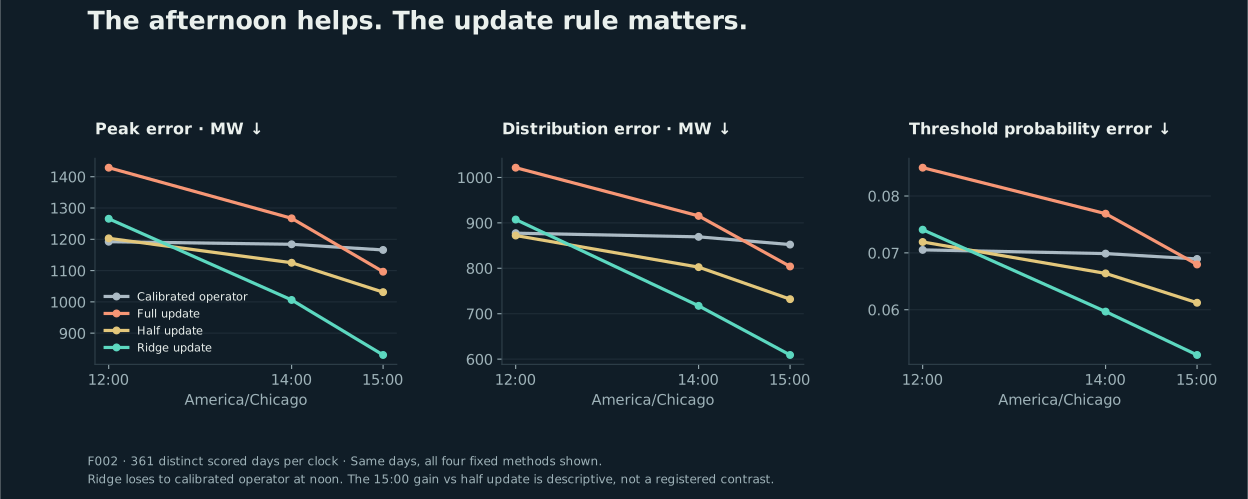
At noon, ridge loses to the calibrated operator. By 15:00, it is the strongest of these four methods on all three reported average scores. The right lesson is to test the information available at each decision time.
MAE measures the average absolute error of the predicted peak; lower is better.
| Clock | Model | MAE MW | CRPS MW | Brier |
|---|
F002 · 361 distinct scored days per clock, not thousands of independent outcomes. The 15:00 ridge-vs-half headline is descriptive and was not a registered inferential contrast. Download the complete three-metric figure.
A nominal 90% range covered only 81.72% of outcomes at 14:00 in the matched ridge control.
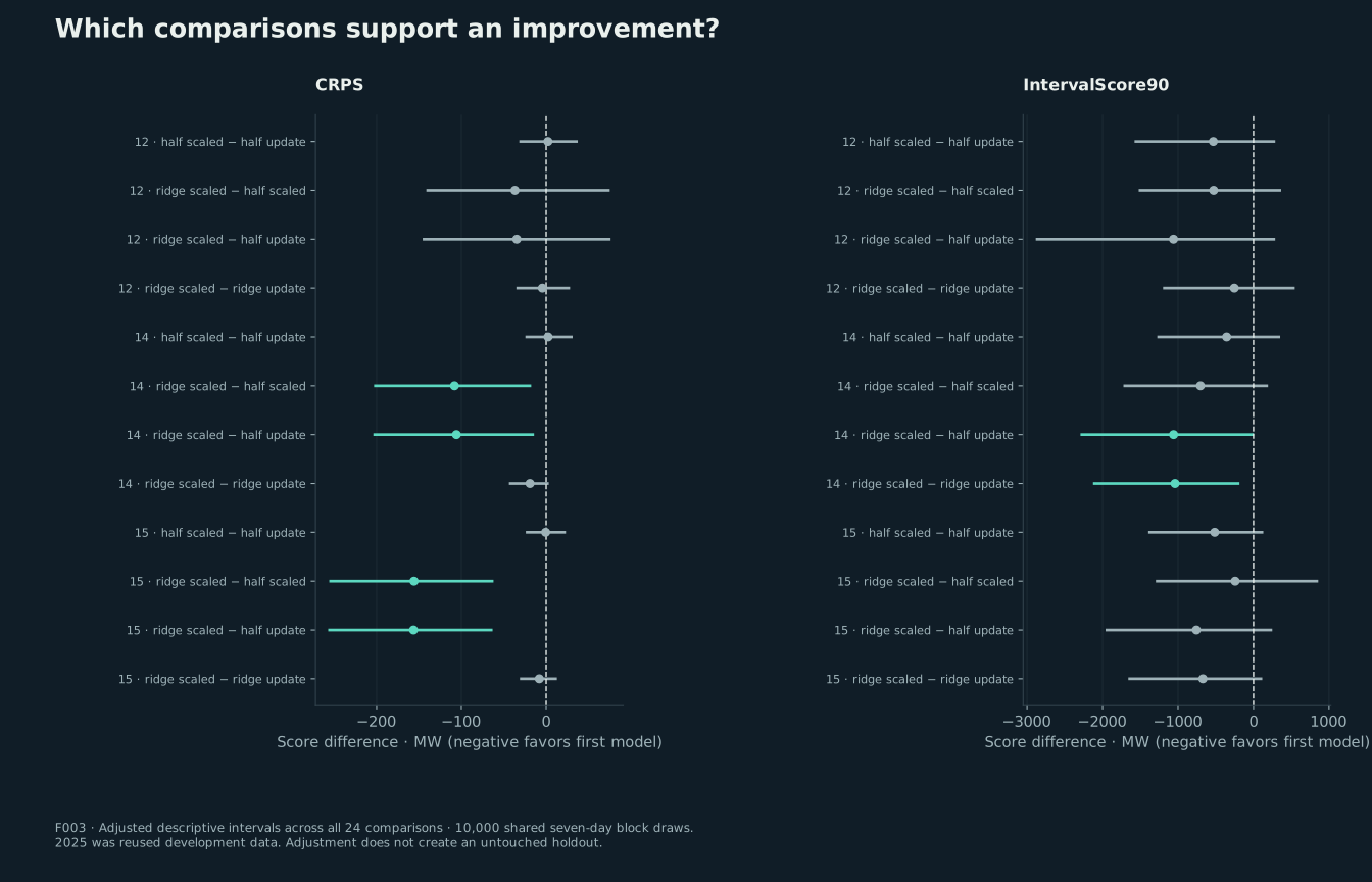
Scaling the residual paths raised coverage to 90.30%. The ranges became 23.07% wider, but a score charging for both width and misses improved by 15.04%.
The improvement was narrower than “the model is calibrated.” Its full-distribution score improvement had an adjusted interval crossing zero. At 15:00, even the scaled nominal 95% interval covered only 91.97% of outcomes.
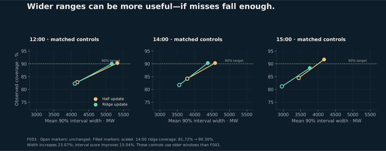
Each month and clock uses separate fitting, donor-library and tuning windows. A scale of 1, 1.25, 1.5 or 2 is chosen before that month’s evaluation. Scale 1—no widening—wins in many folds.
All 24 comparisons are retained. Shared seven-day blocks account for serial dependence when summarizing uncertainty; adjusting the intervals does not make a reused development year an untouched holdout.
Spread each historical hourly error path around the mean path, then take the daily maximum. Hourly means stay fixed; the nonlinear peak’s median can move.
Read the derivation →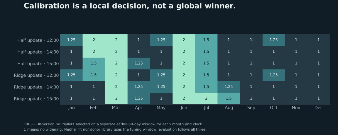
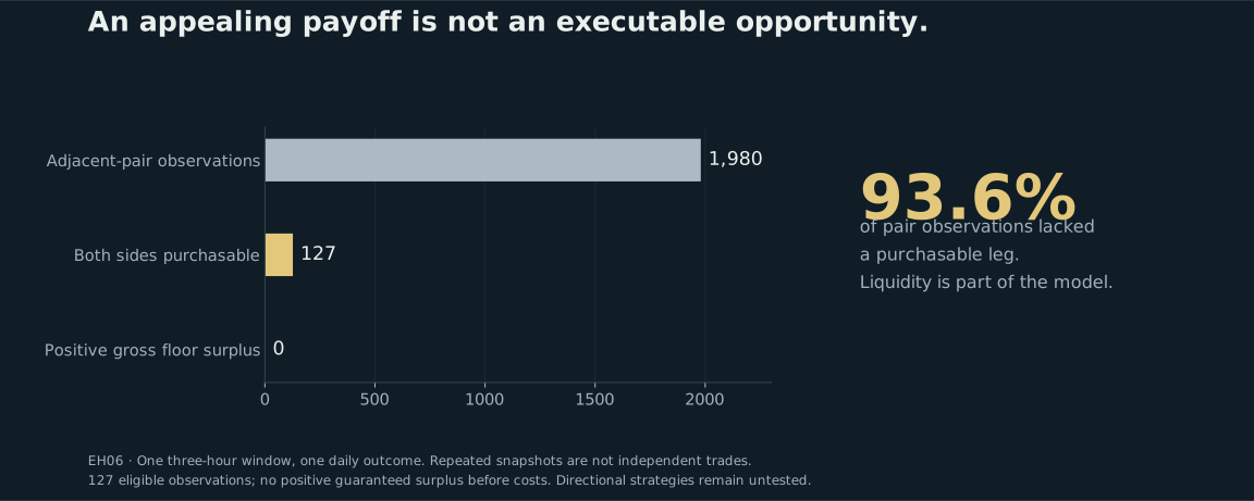
The first price screen found no positive guaranteed package surplus.
For two nested thresholds, YES on the lower threshold plus NO on the higher one pays at least $1 in every outcome. A buy price below $1 would be a necessary first condition for that particular package to lock in gross value.
Across 1,980 adjacent-pair observations, only 127 had both purchasable legs. None passed that condition before costs. These were repeated snapshots of one daily outcome, not 1,980 independent opportunities. This result rejects the observed packages, not every directional strategy.
Three forecast rules × two risk budgets × three execution assumptions. These are parallel policy comparisons, not $3,600 invested.
Zero completed decisions, orders or settlements. No return, win-rate or drawdown claim is available. The first decision is scheduled for 12:00 CT. An overnight quote-recorder failure caused a real coverage gap; recovery is documented separately and does not backfill missed observations.
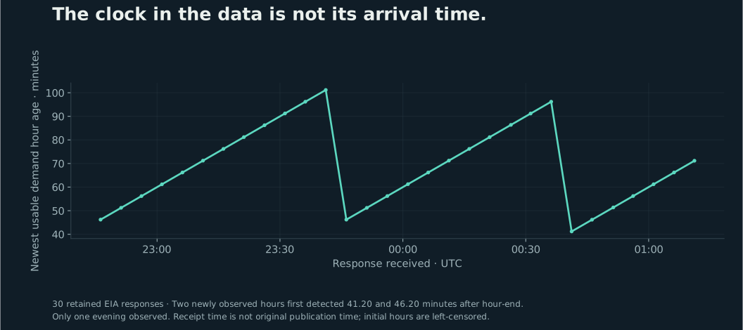
The system records raw response receipts, distinguishes event time from arrival time, freezes experiment definitions and reconstructs outputs independently. Missing inputs and unsuccessful attempts remain visible.
The public repository provides the energy modules, tests, synthetic execution example, retained result reports and chart data. It reproduces the figures and checks the software offline. Full historical experiments additionally require the separately retained raw inputs; the included reports alone cannot reproduce those data acquisitions.
At the publication checkpoint, including the recorder recovery. Network access is denied during the Python test phase. The synthetic demo is explicitly invented data.
The retained F003 independent audit checked predictions, scores, tuning outputs and every bootstrap comparison across 342 artifacts.
Missing forecasts, missing observations and invalid retrospective labels are distinguished. Only 361 days per clock are scored in F002/F003.
Most of the initial improvement came from removing bias. Any complex model should clear that stronger baseline before claiming useful incremental skill.
Peak error, probability quality, interval calibration and realized net return answer different questions. An improvement in one does not settle the others.
The gas-storage alternative remained blocked by original-release and executable-price data. Wholesale electricity spreads require a separate access route. Neither is a validated result here.
The current contribution is an auditable forecasting and execution research system. A tradable edge still needs timestamp-correct input and quote overlap, independent evaluation and forward fills.
Project design, implementation and research direction by Martin Mashalov, developed with AI coding and research assistance. The methods are established statistical tools; the contribution is their integration, measurement and audit trail.